7 Timezones

7.1 Timezone Effect on Team Performance

Code

library(dplyr)
library(ggplot2)
library(scales)
scores <- read.csv("data/2023NFLSCORES.csv")
scores <- scores %>%
  rename(
    Home_Team = X.1,
    Away_Team = X.2,
    Home_Score = X.4,
    Away_Score = X.3
  )
team_tz <- data.frame(
  team = c("SEA", "SF", "LAR", "LAC", "LAV", "DEN", "ARI", "MIN","KC", "DAL", "HOU", "NO", "TEN", "CHI", "GB", "IND", "DL", "CLE", "ATL", "CAR","JAX", "TB", "MIA", "PIT", "BUF", "BAL", "PHI", "NYJ", "NYG", "NE", "CIN", "WAS" 
  ),
  timezone = c("PST", "PST", "PST", "PST","PST", "MT", "MT", "CT", "CT", "CT", "CT", "CT", "CT", "CT", "CT", "ET", "ET", "ET", "ET", "ET", "ET", "ET", "ET", "ET", "ET", "ET", "ET", "ET", "ET", "ET", "ET", "ET" 
               )
)

tz_map <- c(PST = -3, MT = -2, CT = -1, ET = 0)


games <- scores %>%
  left_join(team_tz, by = c('Home_Team' = 'team')) %>%
  rename(home_tz = timezone) %>%
  left_join(team_tz, by = c('Away_Team' = 'team'))%>%
  rename(away_tz = timezone)

games <- games %>%
  mutate(
    Home_Score = as.numeric(Home_Score),
    Away_Score = as.numeric(Away_Score),
    home_offset = tz_map[home_tz],
    away_offset = tz_map[away_tz],
    tz_diff = abs(home_offset - away_offset),
    point_diff = Away_Score - Home_Score,
  )

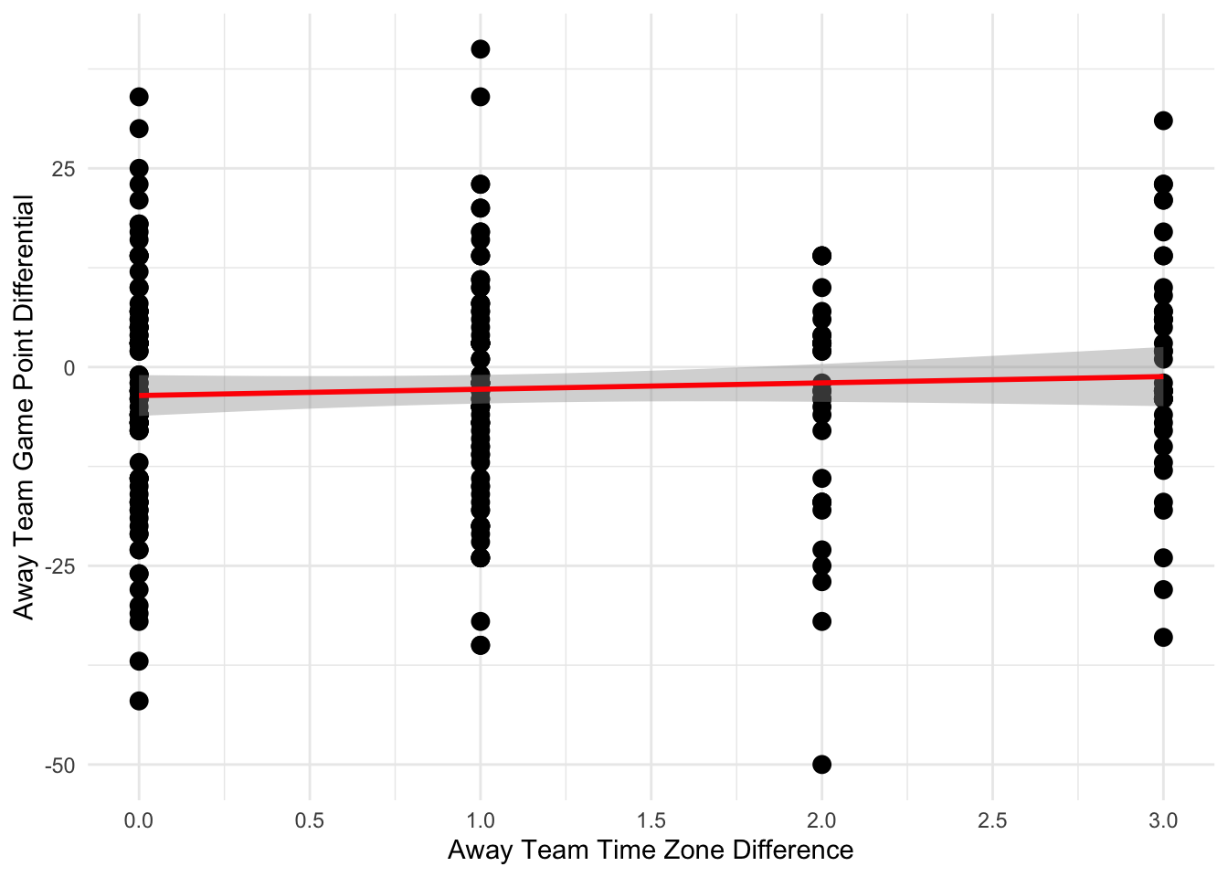
ggplot(games, aes(x = tz_diff, y = point_diff)) + geom_point(size = 3) + geom_smooth(method = "lm", se = TRUE, color = 'red') + theme_minimal() +
  scale_x_continuous(breaks = pretty_breaks()) + labs(
    x = 'Away Team Time Zone Difference',
    y = 'Away Team Game Point Differential'
  )

Another aspect of the schedule we were interested in was how travel affected the performance of teams. In order to look at this, we plotted the point differential of the away team and the home team against the time zone difference the away team faced. The linear regression line has a slope of .79 for every time zone crossed, indicating that with every timezone we cross, we might expect the away team to score .79 more points per game, to our surprise. However, the 95% confidence interval ranges from (-.90 , 2.49) meaning that we cannot be confident our slope is non-zero or even positive. Overall this shows that teams traveling farther for their matches do not perform noticeably worse. Eagles fans shouldn’t be more worried about a game in San Francisco compared to Tampa Bay. However, we did find that there was a negative intercept of -3.58 with a 95% confidence interval ranging from (-6.15, -1.00), meaning we can be confident that our intercept is indeed negative. This negative intercept for a point differential at an away game means that on average away teams in 2023 performed worse than home teams.

This is what we would expect with the results, as it is generally known that home teams have an advantage. Beyond just a win record, we can see that blowouts are more likely to occur from home teams as well. From the graph, there were 6 games where the home team lost by 25 or more points. We can compare that with away teams which were blown out by 25 points or more 15 times over the regular season, one of which was by 50 points (Miami Dolphins hosting the Denver Broncos).

7.2 Linear Regression Outputs

Code

m <- lm(point_diff ~ tz_diff, data = games)
coef(m)["tz_diff"]

  tz_diff 
0.7947086

Code

confint(m, "tz_diff", level = 0.95)

             2.5 %   97.5 %
tz_diff -0.9045339 2.493951

Code

coef(m)["(Intercept)"]

(Intercept) 
   -3.58004

Code

confint(m, "(Intercept)", level = 0.95)

                2.5 %    97.5 %
(Intercept) -6.152858 -1.007222