3  Results

3.1 Offensive Formation vs Defensive Coverage Effectiveness

One thing we’d like to use this data to understand is which types of situations are advantageous for offenses when it comes to playcalling. Can we find out which offensive formations are most likely to be successful, especially if we know the opposing team has a tendency to call a specific defensive coverage?

library(ggplot2)
library(dplyr)
library(reticulate)
library(tidyr)


in_week1 <- read.csv("data/train/input_2023_w01.csv")
in_week2 <- read.csv("data/train/input_2023_w02.csv")
in_week3 <- read.csv("data/train/input_2023_w03.csv")
in_week4 <- read.csv("data/train/input_2023_w04.csv")
in_week5 <- read.csv("data/train/input_2023_w05.csv")
in_week6 <- read.csv("data/train/input_2023_w06.csv")
in_week7 <- read.csv("data/train/input_2023_w07.csv")
in_week8 <- read.csv("data/train/input_2023_w08.csv")
in_week9 <- read.csv("data/train/input_2023_w09.csv")
in_week10 <- read.csv("data/train/input_2023_w10.csv")
in_week11 <- read.csv("data/train/input_2023_w11.csv")
in_week12 <- read.csv("data/train/input_2023_w12.csv")
in_week13 <- read.csv("data/train/input_2023_w13.csv")
in_week14 <- read.csv("data/train/input_2023_w14.csv")
in_week15 <- read.csv("data/train/input_2023_w15.csv")
in_week16 <- read.csv("data/train/input_2023_w16.csv")
in_week17 <- read.csv("data/train/input_2023_w17.csv")
in_week18 <- read.csv("data/train/input_2023_w18.csv")


out_week1 <- read.csv("data/train/output_2023_w01.csv")
out_week2 <- read.csv("data/train/output_2023_w02.csv")
out_week3 <- read.csv("data/train/output_2023_w03.csv")
out_week4 <- read.csv("data/train/output_2023_w04.csv")
out_week5 <- read.csv("data/train/output_2023_w05.csv")
out_week6 <- read.csv("data/train/output_2023_w06.csv")
out_week7 <- read.csv("data/train/output_2023_w07.csv")
out_week8 <- read.csv("data/train/output_2023_w08.csv")
out_week9 <- read.csv("data/train/output_2023_w09.csv")
out_week10 <- read.csv("data/train/output_2023_w10.csv")
out_week11 <- read.csv("data/train/output_2023_w11.csv")
out_week12 <- read.csv("data/train/output_2023_w12.csv")
out_week13 <- read.csv("data/train/output_2023_w13.csv")
out_week14 <- read.csv("data/train/output_2023_w14.csv")
out_week15 <- read.csv("data/train/output_2023_w15.csv")
out_week16 <- read.csv("data/train/output_2023_w16.csv")
out_week17 <- read.csv("data/train/output_2023_w17.csv")
out_week18 <- read.csv("data/train/output_2023_w18.csv")

supplementary <- read.csv("data/supplementary_data.csv")

# Create offense_win_probability_added and defense_win_probability_added columns
# Logic: If possession_team == home_team, offense gets home WPA, defense gets visitor WPA
#        If possession_team == visitor_team, offense gets visitor WPA, defense gets home WPA

supplementary <- supplementary |>
  mutate(
    offense_win_probability_added = ifelse(
      possession_team == home_team_abbr,
      home_team_win_probability_added,
      visitor_team_win_probility_added
    ),
    defense_win_probability_added = ifelse(
      possession_team == home_team_abbr,
      visitor_team_win_probility_added,
      home_team_win_probability_added
    )
  )

# Remove NA values for the variables we're plotting
supp_clean <- supplementary |>
  filter(!is.na(offense_formation) &
         !is.na(team_coverage_type) &
         !is.na(expected_points_added) &
         !is.na(offense_win_probability_added))

# Get all unique combinations of offense_formation and team_coverage_type
formations <- unique(supp_clean$offense_formation)
coverages <- unique(supp_clean$team_coverage_type)

3.1.1 Scatterplot of each formation vs coverage combination and their respective EPA vs Win Probability Added

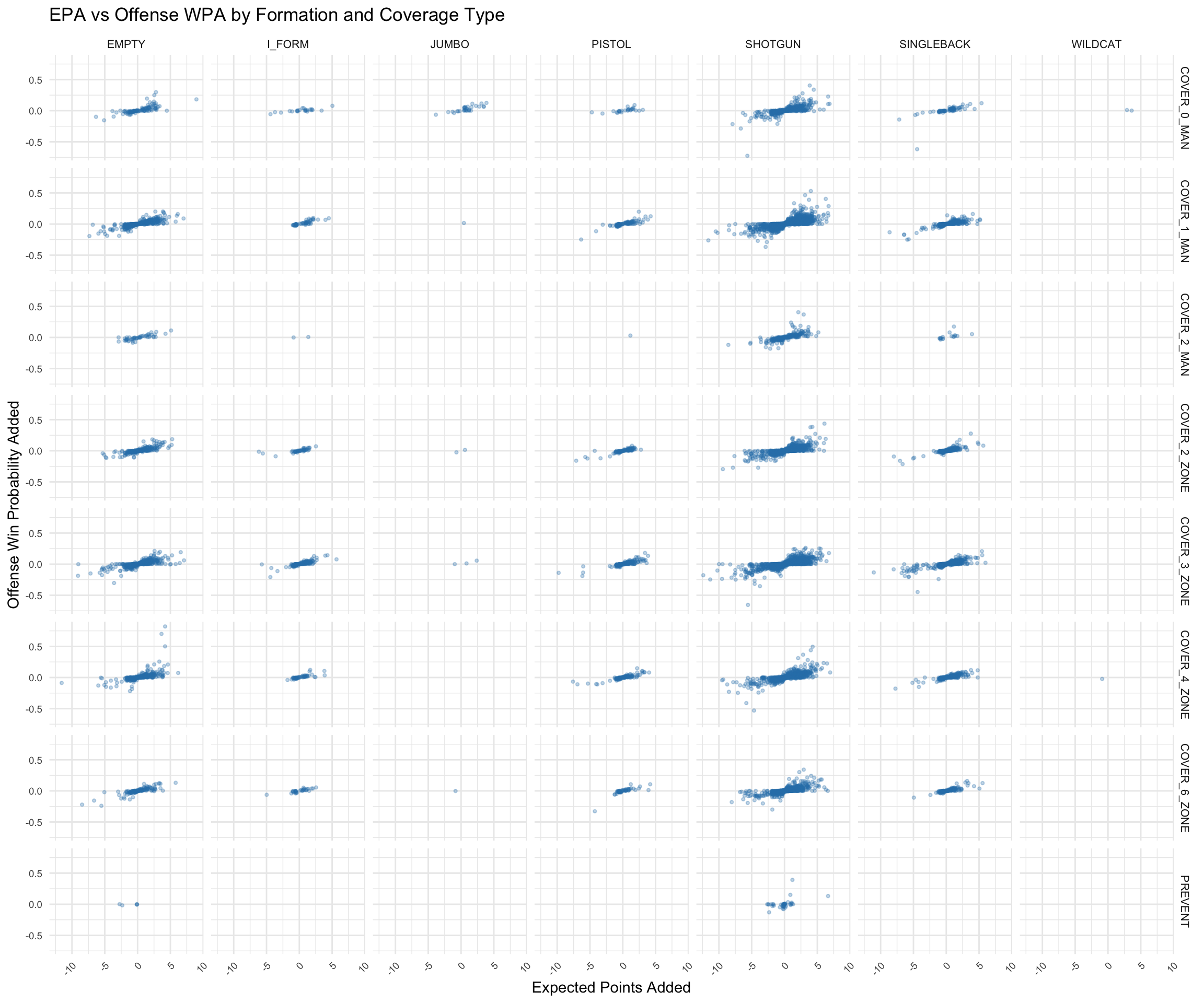
The first thing we can do to answer this question is view every combination of offensive formation and defensive coverage and get a general sense of both the frequency with which each combination occurs, as well as how generally successful that combination tends to be.

# Create a faceted scatter plot for all combinations
ggplot(supp_clean, aes(x = expected_points_added, y = offense_win_probability_added)) +
  geom_point(alpha = 0.3, size = 0.8, color = "#2c7fb8") +
  facet_grid(team_coverage_type ~ offense_formation) +
  labs(
    title = "EPA vs Offense WPA by Formation and Coverage Type",
    x = "Expected Points Added",
    y = "Offense Win Probability Added"
  ) +
  theme_minimal() +
  theme(
    axis.text.x = element_text(angle = 45, hjust = 1, size = 7),
    axis.text.y = element_text(size = 7),
    strip.text = element_text(size = 8)
  )

The above shows a grid of scatterplots for every possible offensive formation against every possible defensive coverage, and shows the Expected Points Added (EPA) as well as Offensive Win Probability Added (WPA). This gives us an idea of which offensive/defensive combinations occur most frequently. We also see that every scatterplot has a relatively strong positive correlation, which aligns with our intuition that if a play has a positive amount of expected points added, it also gives the offensive team a higher win probability. However, it’s a bit difficult to tell any more specific information from this plot, so lets dive a bit deeper:

3.1.2 Formation vs Coverage EPA Boxplots

# Create a combined factor for formation-coverage pairs
supp_clean <- supp_clean |>
  mutate(formation_coverage = paste(offense_formation, team_coverage_type, sep = " vs "))

# Filter to only include combinations with at least 100 plays
supp_filtered <- supp_clean |>
  group_by(formation_coverage) |>
  filter(n() >= 100) |>
  ungroup()

# Calculate median EPA for each combination to order them
median_epa <- supp_filtered |>
  group_by(formation_coverage) |>
  summarise(median_epa = median(expected_points_added, na.rm = TRUE)) |>
  arrange(desc(median_epa))

# Reorder the factor based on median EPA
supp_filtered$formation_coverage <- factor(supp_filtered$formation_coverage,
                                         levels = median_epa$formation_coverage)

# Create boxplots
ggplot(supp_filtered, aes(x = formation_coverage, y = expected_points_added)) +
  geom_boxplot(fill = "#2c7fb8", alpha = 0.7, outlier.alpha = 0.3, outlier.size = 0.5) +
  geom_hline(yintercept = 0, linetype = "dashed", color = "red", linewidth = 0.5) +
  labs(
    title = "Expected Points Added by Formation and Coverage Type",
    subtitle = "Ordered by median EPA (descending)",
    x = "Formation vs Coverage Combination",
    y = "Expected Points Added"
  ) +
  theme_minimal() +
  theme(
    axis.text.x = element_text(angle = 90, hjust = 1, vjust = 0.5, size = 7),
    axis.text.y = element_text(size = 8),
    panel.grid.major.x = element_blank()
  )

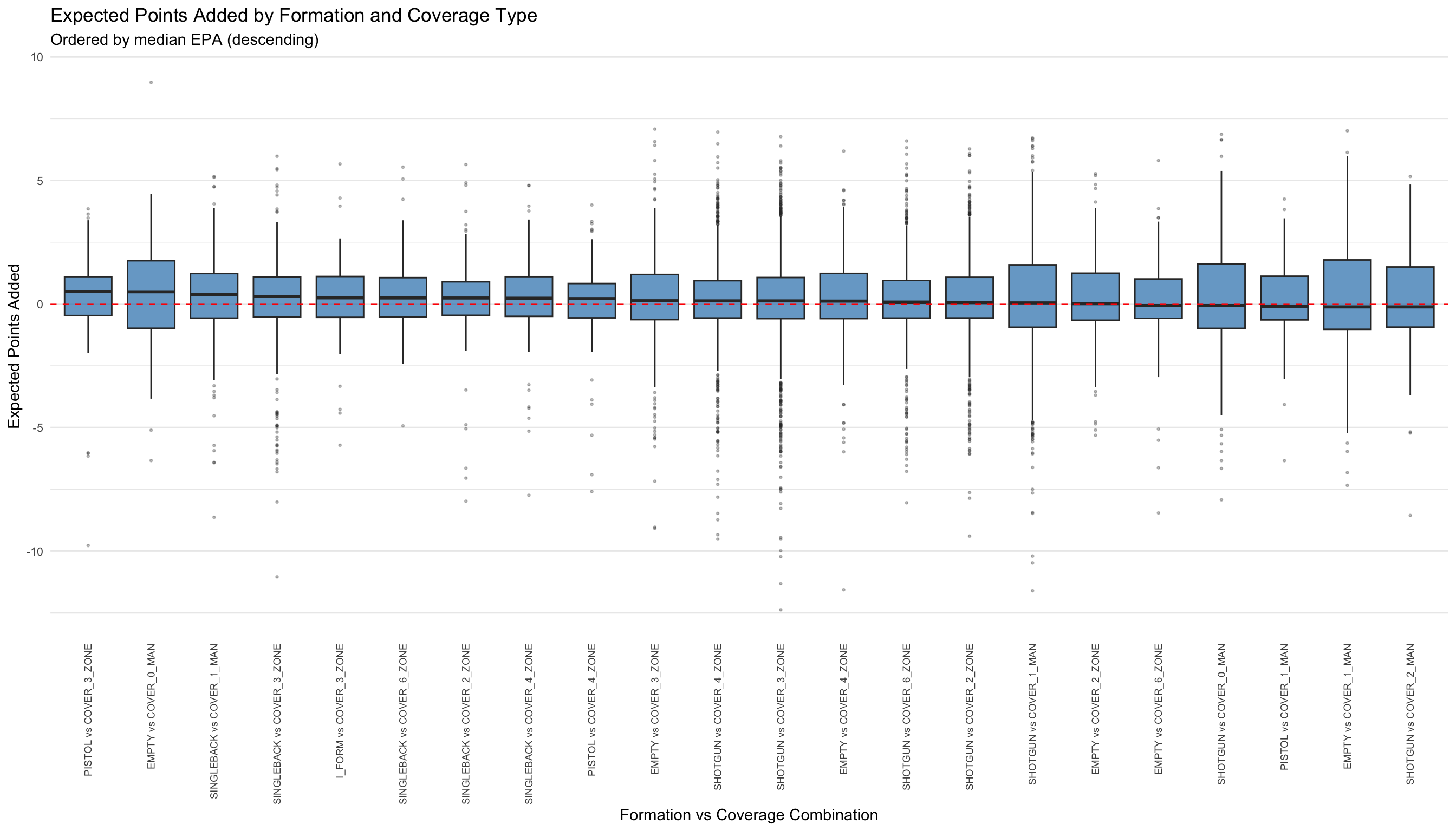
In the above, we have box plots of Offensive Formation/Defensive Coverage combos, sorted by descending mean EPA per play – we no longer need to look at WPA, as we have concluded that EPA and WPA are strongly correlated and redundant. We have filtered to only show combinations that have occurred 100 times of more throughout the season.

This chart makes it a bit easier for us to understand some key takeaways. Firstly, we see that the single most successful Offensive Formation/Defensive Coverage combination (where success is measured in terms of Offensive EPA) is the Pistol Formation vs Cover 3 Zone. We also see that Shotgun vs Cover 2 Man is the worst combination for the offense to find itself in, which, on average, contributes a negative EPA.

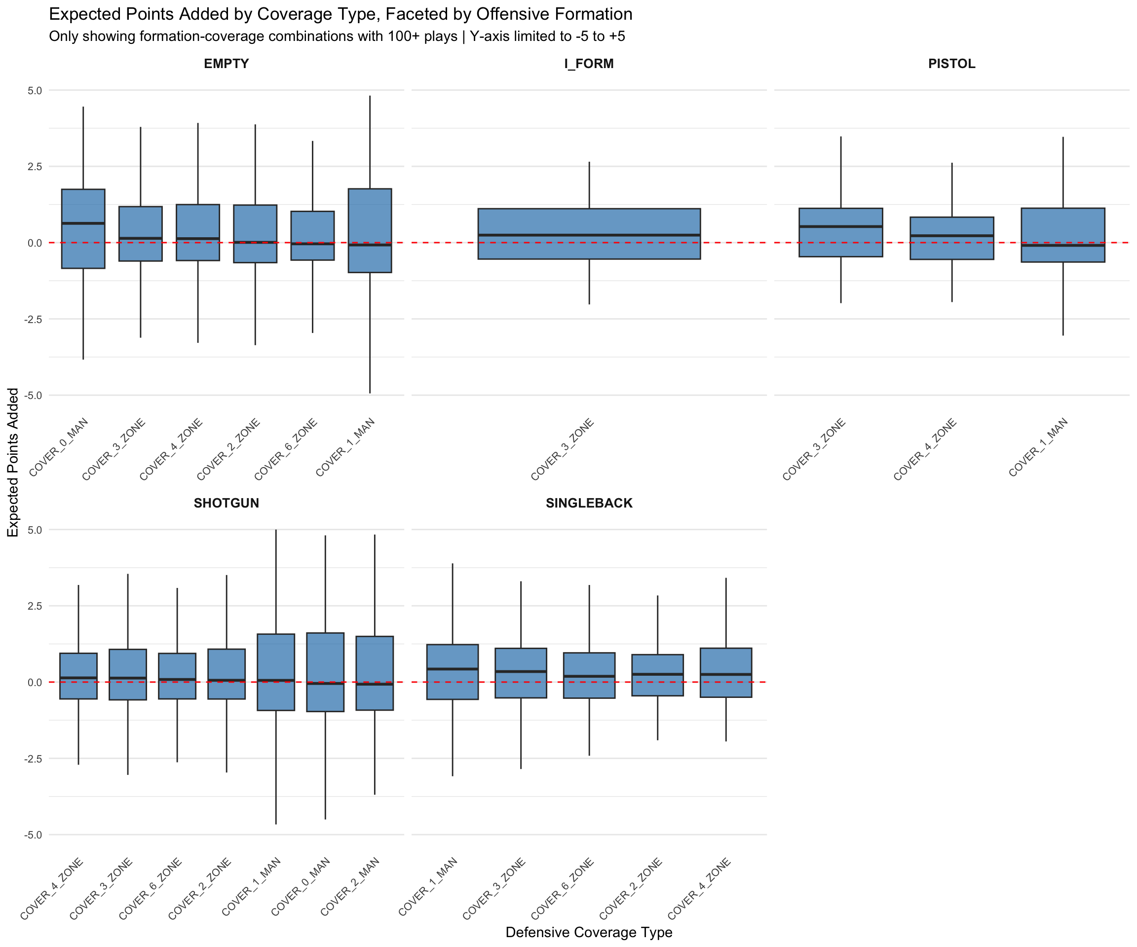
However, it is still a bit tricky to really make sense of how individual offensive formations perform against each other when seeing different devensive coverages, and which offensive formations are generally most effective, regardless of defensive formation. To address this, we can facet the box plots by offensive formation and look a little closer:

3.1.3 Faceted Boxplots by Offensive Formation

# Create a combined factor for formation-coverage pairs
supp_clean <- supp_clean |>
  mutate(formation_coverage = paste(offense_formation, team_coverage_type, sep = " vs "))

# Filter to only include combinations with at least 100 plays
supp_filtered <- supp_clean |>
  group_by(formation_coverage) |>
  filter(n() >= 100) |>
  ungroup()

# Split data by offensive formation
formation_list <- split(supp_filtered, supp_filtered$offense_formation)

# Process each formation subtable separately
formation_list_processed <- lapply(formation_list, function(formation_df) {
  formation_name <- unique(formation_df$offense_formation)

  # Calculate median EPA for each coverage type within this formation
  formation_df <- formation_df |>
    group_by(team_coverage_type) |>
    mutate(median_epa = median(expected_points_added, na.rm = TRUE)) |>
    ungroup()

  # Create ordered factor for coverage type based on median EPA
  # Use concatenated string to make unique factor levels per formation
  coverage_order <- formation_df |>
    group_by(team_coverage_type) |>
    summarise(median_epa = first(median_epa)) |>
    arrange(desc(median_epa)) |>
    mutate(coverage_concat = paste(team_coverage_type, formation_name, sep = "___")) |>
    pull(coverage_concat)

  # Create concatenated coverage identifier
  formation_df$coverage_concat <- paste(formation_df$team_coverage_type,
                                        formation_name,
                                        sep = "___")

  # Set factor levels with formation-specific ordering
  formation_df$coverage_ordered <- factor(formation_df$coverage_concat,
                                          levels = coverage_order)

  return(formation_df)
})

# Combine all formation subtables back together
supp_filtered_ordered <- bind_rows(formation_list_processed)

# Create a labeller function to strip the formation suffix from labels
strip_formation <- function(x) {
  gsub("___.*$", "", x)
}

# Create faceted boxplots
ggplot(supp_filtered_ordered, aes(x = coverage_ordered, y = expected_points_added)) +
  geom_boxplot(fill = "#2c7fb8", alpha = 0.7, outlier.shape = NA) +
  geom_hline(yintercept = 0, linetype = "dashed", color = "red", linewidth = 0.5) +
  facet_wrap(~ offense_formation, scales = "free_x") +
  scale_x_discrete(labels = strip_formation) +
  scale_y_continuous(limits = c(-5, 5)) +
  labs(
    title = "Expected Points Added by Coverage Type, Faceted by Offensive Formation",
    subtitle = "Only showing formation-coverage combinations with 100+ plays | Y-axis limited to -5 to +5",
    x = "Defensive Coverage Type",
    y = "Expected Points Added"
  ) +
  theme_minimal() +
  theme(
    axis.text.x = element_text(angle = 45, hjust = 1, size = 8),
    axis.text.y = element_text(size = 8),
    strip.text = element_text(size = 10, face = "bold"),
    panel.grid.major.x = element_blank()
  )

From the above, we can see a few interesting trends.

One that immediately jumps out is that the Singleback formation is the only offensive formation (with the exception of I Formation, which only has enough data against one formation) where the average EPA is positive against every common defensive coverage it faces.

Another thing we notice here is that Cover 3 Zone is a top 2 formation in terms of EPA allowed against every offensive formation we see here, indicating that no matter which formation the offense comes out in, they would be happy to see themselves playing against a Cover 3 Zone formation.

Lastly, we can see that the Pistol formation seems to be a bit higher risk, higher reward than our other formations, with the top overall formation/coverage combination (when going against Cover 3 Zone), but also one of the lowest performing combinations (when going against Cover 1 Man).