4  Results (continued)

4.1 Receiver Separation Analysis

Another topic that we’d like to explore with this data set is Targeted Receiver Separation from Defenders. We’d like to find out which route runners are most effective at creating space to get open, as well as explore whether Play Action passing has a positive effect on generating more open receivers.

To start, we need to manipulate our data to calculate the nearest defender to the targeted receiver for every play in our dataset, then group the plays together by the targeted receiver so that we can see which route runners are best at getting open:

Code
library(ggplot2)
library(dplyr)
library(reticulate)
library(lubridate)

in_week1 <- read.csv("data/train/input_2023_w01.csv")
in_week2 <- read.csv("data/train/input_2023_w02.csv")
in_week3 <- read.csv("data/train/input_2023_w03.csv")
in_week4 <- read.csv("data/train/input_2023_w04.csv")
in_week5 <- read.csv("data/train/input_2023_w05.csv")
in_week6 <- read.csv("data/train/input_2023_w06.csv")
in_week7 <- read.csv("data/train/input_2023_w07.csv")
in_week8 <- read.csv("data/train/input_2023_w08.csv")
in_week9 <- read.csv("data/train/input_2023_w09.csv")
in_week10 <- read.csv("data/train/input_2023_w10.csv")
in_week11 <- read.csv("data/train/input_2023_w11.csv")
in_week12 <- read.csv("data/train/input_2023_w12.csv")
in_week13 <- read.csv("data/train/input_2023_w13.csv")
in_week14 <- read.csv("data/train/input_2023_w14.csv")
in_week15 <- read.csv("data/train/input_2023_w15.csv")
in_week16 <- read.csv("data/train/input_2023_w16.csv")
in_week17 <- read.csv("data/train/input_2023_w17.csv")
in_week18 <- read.csv("data/train/input_2023_w18.csv")

out_week1 <- read.csv("data/train/output_2023_w01.csv")
out_week2 <- read.csv("data/train/output_2023_w02.csv")
out_week3 <- read.csv("data/train/output_2023_w03.csv")
out_week4 <- read.csv("data/train/output_2023_w04.csv")
out_week5 <- read.csv("data/train/output_2023_w05.csv")
out_week6 <- read.csv("data/train/output_2023_w06.csv")
out_week7 <- read.csv("data/train/output_2023_w07.csv")
out_week8 <- read.csv("data/train/output_2023_w08.csv")
out_week9 <- read.csv("data/train/output_2023_w09.csv")
out_week10 <- read.csv("data/train/output_2023_w10.csv")
out_week11 <- read.csv("data/train/output_2023_w11.csv")
out_week12 <- read.csv("data/train/output_2023_w12.csv")
out_week13 <- read.csv("data/train/output_2023_w13.csv")
out_week14 <- read.csv("data/train/output_2023_w14.csv")
out_week15 <- read.csv("data/train/output_2023_w15.csv")
out_week16 <- read.csv("data/train/output_2023_w16.csv")
out_week17 <- read.csv("data/train/output_2023_w17.csv")
out_week18 <- read.csv("data/train/output_2023_w18.csv")

supplementary <- read.csv("data/supplementary_data.csv")

# Combine all weekly input data
all_weeks <- bind_rows(
  in_week1, in_week2, in_week3, in_week4, in_week5, in_week6,
  in_week7, in_week8, in_week9, in_week10, in_week11, in_week12,
  in_week13, in_week14, in_week15, in_week16, in_week17, in_week18
)

# For each play, get the final frame (ball arrival)
ball_arrival_frames <- all_weeks |>
  group_by(game_id, play_id) |>
  summarise(arrival_frame = max(frame_id), .groups = "drop")

# Filter to ball arrival frame
all_weeks_ball_arrival <- all_weeks |>
  inner_join(ball_arrival_frames, by = c("game_id", "play_id")) |>
  filter(frame_id == arrival_frame)

# Get defenders at ball arrival
defenders <- all_weeks_ball_arrival |>
  filter(player_role == "Defensive Coverage") |>
  select(game_id, play_id, nfl_id, x, y) |>
  rename(defender_id = nfl_id, defender_x = x, defender_y = y)

# Get only targeted receivers at ball arrival
# (excluding other route runners to avoid inflated separation from defenders moving toward target)
receivers_and_runners <- all_weeks_ball_arrival |>
  filter(player_role == "Targeted Receiver") |>
  select(game_id, play_id, frame_id, nfl_id, x, y, player_role, player_position)

# Calculate nearest defender for each targeted receiver
nearest_defenders <- receivers_and_runners |>
  inner_join(defenders, by = c("game_id", "play_id"), relationship = "many-to-many") |>
  mutate(distance = sqrt((x - defender_x)^2 + (y - defender_y)^2)) |>
  group_by(game_id, play_id, frame_id, nfl_id) |>
  slice_min(distance, n = 1, with_ties = FALSE) |>
  ungroup() |>
  select(game_id, play_id, frame_id, nfl_id,
         nearest_defender_id = defender_id,
         nearest_defender_distance = distance)

# Add nearest_defender_id and nearest_defender_distance columns to all_weeks
all_weeks <- all_weeks |>
  left_join(nearest_defenders, by = c("game_id", "play_id", "frame_id", "nfl_id"))

# Filter all_weeks to only include rows where nearest_defender columns are not NA
# (i.e., only receivers/route runners)
all_weeks_filtered <- all_weeks |>
  filter(!is.na(nearest_defender_id) & !is.na(nearest_defender_distance))


# Replace all_weeks with the filtered version
all_weeks <- all_weeks_filtered

# Calculate average separation per receiver
# Group by nfl_id and player name, count routes, and calculate average separation
receiver_separation <- all_weeks |>
  filter(player_position == "WR") |>
  group_by(nfl_id, player_name, player_position) |>
  summarise(
    routes_ran = n_distinct(paste(game_id, play_id)),
    avg_separation = mean(nearest_defender_distance, na.rm = TRUE),
    .groups = "drop"
  ) |>
  filter(routes_ran >= 50) |>
  arrange(desc(avg_separation)) |>
  head(10)

# Create a bar plot
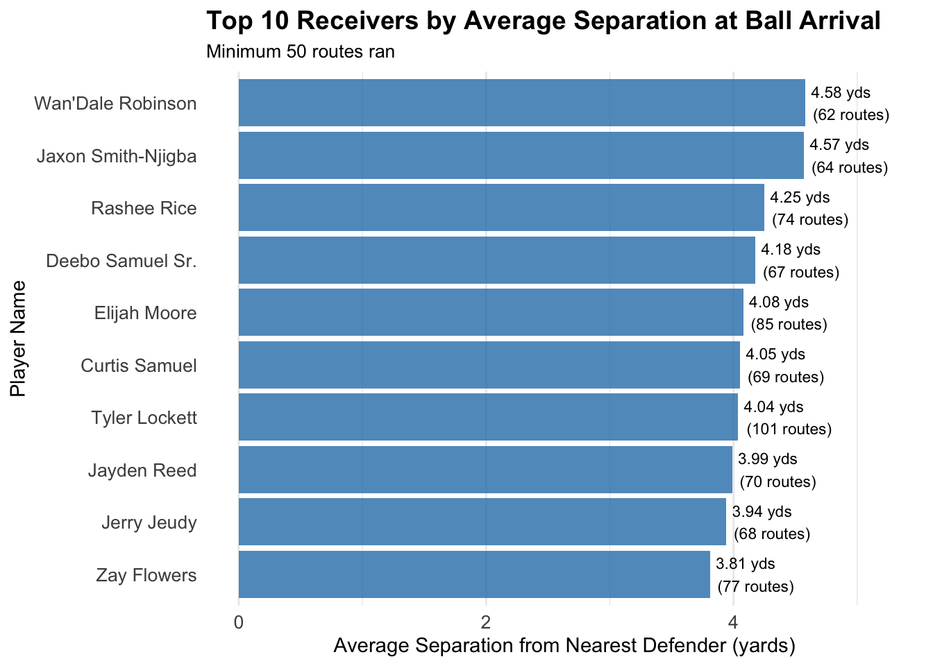
ggplot(receiver_separation, aes(x = reorder(player_name, avg_separation), y = avg_separation)) +
  geom_bar(stat = "identity", fill = "#2c7fb8", alpha = 0.8) +
  geom_text(aes(label = paste0(round(avg_separation, 2), " yds\n(", routes_ran, " routes)")),
            hjust = -0.1, size = 3) +
  coord_flip() +
  labs(
    title = "Top 10 Receivers by Average Separation at Ball Arrival",
    subtitle = "Minimum 50 routes ran",
    x = "Player Name",
    y = "Average Separation from Nearest Defender (yards)"
  ) +
  theme_minimal() +
  theme(
    plot.title = element_text(face = "bold", size = 14),
    plot.subtitle = element_text(size = 10),
    axis.text = element_text(size = 10),
    panel.grid.major.y = element_blank()
  ) +
  ylim(0, max(receiver_separation$avg_separation) * 1.15)

From the above, we can see the top 10 WRs from the 2023 NFL season in terms of getting open. We made sure to filter out players with under 50 targets so that we only include wideouts that have a reasonable sample size of targets. Unsurprisingly, the list contains many names of known speedsters across the league – players notable for their elite quickness. Players like Wan’Dale Robinson, Rashee Rice, Tyler Lockett, and Jayden Reed are all known for their deep-ball prominence and being able to get past the defense with their speed.

4.2 Play Action Effect on Receiver Separation by Route Type

One other aspect to analyze in this area is whether Play Action Pass (plays where the quarterback initially fakes a handoff to the runningback, but keeps the ball to then throw to a receiver) truly has a significant impact on being able to scheme receivers open for NFL offenses.

However, we need to be somewhat careful with this analysis – play action play design can have a tendency to use some route types (Slant, Go, Post, Dig, etc.) significantly more than others, and different routes can have inherently different expectations for level of separation generated. So, in order to properly demonstrate this effect, we want to first facet by route type for each targeted pass, resulting in several different plots that show the rough densities of separation gained by the receiver in Play Action vs Standard passing plays:

Code
# Join all_weeks with supplementary data to get play_action and route information
all_weeks_with_play_info <- all_weeks |>
  inner_join(
    supplementary |> select(game_id, play_id, play_action, route_of_targeted_receiver),
    by = c("game_id", "play_id")
  ) |>
  filter(
    !is.na(play_action),
    !is.na(route_of_targeted_receiver),
    !is.na(nearest_defender_distance),
    player_position == "WR"  # Only wide receivers
  )

# Filter to routes with sufficient sample size (at least 100 observations)
route_counts <- all_weeks_with_play_info |>
  group_by(route_of_targeted_receiver) |>
  summarise(n = n()) |>
  filter(n >= 100)

all_weeks_filtered <- all_weeks_with_play_info |>
  filter(route_of_targeted_receiver %in% route_counts$route_of_targeted_receiver)

# Create overlapping density plots faceted by route type
ggplot(all_weeks_filtered, aes(x = nearest_defender_distance, fill = play_action, color = play_action)) +
  geom_density(alpha = 0.4, linewidth = 0.8) +
  facet_wrap(~ route_of_targeted_receiver, scales = "free_y", ncol = 3) +
  scale_fill_manual(
    values = c("TRUE" = "#d95f02", "FALSE" = "#1b9e77"),
    labels = c("FALSE" = "No Play Action", "TRUE" = "Play Action")
  ) +
  scale_color_manual(
    values = c("TRUE" = "#d95f02", "FALSE" = "#1b9e77"),
    labels = c("FALSE" = "No Play Action", "TRUE" = "Play Action")
  ) +
  labs(
    title = "Effect of Play Action on WR Separation at Ball Arrival by Route Type",
    subtitle = "Targeted receivers only | Routes with 100+ observations",
    x = "Separation from Nearest Defender (yards)",
    y = "Density",
    fill = "Play Type",
    color = "Play Type"
  ) +
  theme_minimal() +
  theme(
    plot.title = element_text(face = "bold", size = 14),
    plot.subtitle = element_text(size = 10),
    strip.text = element_text(face = "bold", size = 9),
    legend.position = "bottom",
    axis.text = element_text(size = 8)
  )

From the above density plots, we can see that for most route types, there is generally a higher frequency of plays that have a low level of separation when the play type is standard, compared to play action. This indicates that play action does positively impact receiver separation from nearest defender, generally speaking. To get a more specific understanding, we can take a look at the overall average separation for each route type, filtered on Play Action vs Standard, and plot it as a Cleveland Dot Plot:

4.2.1 Cleveland Dot Plot: Separation by Route Type and Play Action

Code
# Calculate summary statistics by route and play action
separation_summary <- all_weeks_filtered |>
  group_by(route_of_targeted_receiver, play_action) |>
  summarise(
    n = n(),
    mean_separation = mean(nearest_defender_distance, na.rm = TRUE),
    median_separation = median(nearest_defender_distance, na.rm = TRUE),
    sd_separation = sd(nearest_defender_distance, na.rm = TRUE),
    .groups = "drop"
  ) |>
  arrange(route_of_targeted_receiver, play_action)

# Add play action labels
separation_summary <- separation_summary |>
  mutate(play_action_label = ifelse(play_action == TRUE, "Play Action", "No Play Action"))
# Get play action separation for ordering
pa_order <- separation_summary |>
  filter(play_action == TRUE) |>
  arrange((mean_separation)) |>
  pull(route_of_targeted_receiver)

# Reorder the route factor based on play action separation
separation_summary <- separation_summary |>
  mutate(route_of_targeted_receiver = factor(route_of_targeted_receiver, levels = pa_order))

# Create Cleveland dot plot
ggplot(separation_summary, aes(x = mean_separation, y = route_of_targeted_receiver, color = play_action_label)) +
  geom_line(aes(group = route_of_targeted_receiver), color = "grey70", linewidth = 1) +
  geom_point(size = 4) +
  scale_color_manual(
    values = c("Play Action" = "#d95f02", "No Play Action" = "#1b9e77"),
    name = "Play Type"
  ) +
  labs(
    title = "Average WR Separation by Route Type and Play Action",
    subtitle = "Ordered by Play Action separation (highest to lowest)",
    x = "Mean Separation from Nearest Defender (yards)",
    y = "Route Type"
  ) +
  theme_minimal() +
  theme(
    plot.title = element_text(face = "bold", size = 14),
    plot.subtitle = element_text(size = 10),
    axis.text.y = element_text(size = 10),
    axis.text.x = element_text(size = 10),
    legend.position = "bottom",
    panel.grid.major.y = element_blank(),
    panel.grid.minor.x = element_blank()
  )

Once again, we see that in nearly every case, the Play Action cases of each route type leads to a higher amount of receiver separation from the nearest defender. The only exceptions to this trend are Slant routes and Hitch routes.

Table, for specific values:

Code
print(separation_summary)
# A tibble: 20 × 7
   route_of_targeted_recei…¹ play_action     n mean_separation median_separation
   <fct>                     <lgl>       <int>           <dbl>             <dbl>
 1 CORNER                    FALSE         276            2.88              2.30
 2 CORNER                    TRUE           90            3.30              2.87
 3 CROSS                     FALSE         596            3.74              3.26
 4 CROSS                     TRUE          402            4.51              3.80
 5 FLAT                      FALSE         191            6.06              5.49
 6 FLAT                      TRUE           68            6.47              6.21
 7 GO                        FALSE         949            2.06              1.48
 8 GO                        TRUE          190            2.64              1.73
 9 HITCH                     FALSE        1611            3.82              3.74
10 HITCH                     TRUE          277            3.79              3.35
11 IN                        FALSE         688            3.21              2.90
12 IN                        TRUE          167            3.49              3.16
13 OUT                       FALSE        1212            3.39              3.14
14 OUT                       TRUE          226            3.68              3.24
15 POST                      FALSE         441            2.85              2.49
16 POST                      TRUE          183            3.17              2.63
17 SCREEN                    FALSE         116            8.44              8.69
18 SCREEN                    TRUE           34            9.53              8.89
19 SLANT                     FALSE         787            3.03              2.47
20 SLANT                     TRUE           73            2.81              2.36
# ℹ abbreviated name: ¹​route_of_targeted_receiver
# ℹ 2 more variables: sd_separation <dbl>, play_action_label <chr>